What do you do when you want to use the same column information in multiple Google Sheets? Copy and paste data can only solve the problem temporarily, but when the original data is changed, you have to find the particular sheets that use the original data and make the changes manually. In fact, I am going to share with you a shortcut to deal with this, it is called “Google Sheets Importrange” formula.
When you can use the Google Sheets Importrange Formula?
If you want to use the same data in multiple spreadsheets, and you’re likely need to modify the content of the data in the future, it is very good to make use of “Importrange” formula in Google Sheets to optimize what you’re looking for.
For an example, when you are doing your employee information such as employee salary using the Google Sheets. If the employee salary is directly input or copied and pasted, each Google Sheets will have to be modified in the future when there is a change of staff. It is so troublesome! However, if you are using the “Importrange” formula, you can automatically synchronize to other Google Sheets by modifying the data in the employee salary. You do not have to change everything manually all the time.
How to use the Google Sheets Importrange Formula?
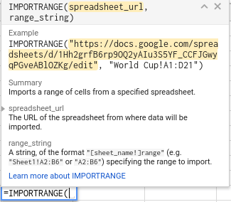
The complete Google Sheets Importrange formula : Importrange “(Employee Salary URL), (Data Range)”. The following steps are explained below.
Step 1. Copy the Google Sheets URL or key value that you want to use
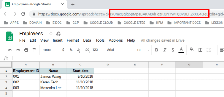
If you want to use”Employees”data and use it in”Salary Calculation”,you can copy all the URLs of the”Employees”or just copy the key value.
※ The key value is a string of English characters from the d/ to /edit, as shown below:
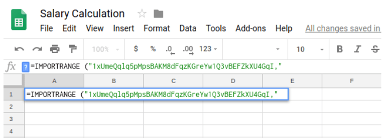
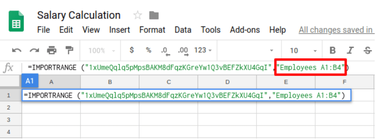
Step 2. Paste the URL or key value into the Importrange formula
Then enter the URL you copied in the Importrange formula, remember to wrap the URL with double quotes“” “”.
Step 3. Enter the range of cells you want to grab
You are free to choose which specific range of cells you want to grab in your”Employees”, but remember to wrap the data in double quotes “” “”.
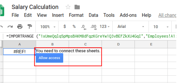
Step 4. Allow the link to Google Sheets
After entering the formula, the”#REF!”error will be displayed. Do not worry! Just click to”Allow Access”button in the figure below and the data will be displayed!
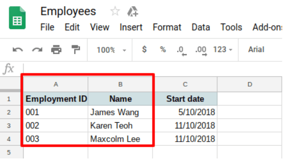
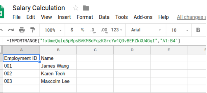
Hence, the”Employee”will be imported into the”Salary Calculation”. In the future, if there is any change in the employee list, the information in the salary calculation sheets will be updated synchronously.
After reading the function of the Google Sheets Importrange Formula, isn’t it is very convenient and easy to use? Try it when you have similar needs next time! It helps you to save the hassle of having to modify the multiple Google Sheet manually.